Introduction
Gridder is a simple interactive grid generation tool for creating orthogonal, structured grids with quadralateral (2D) or hexahedral (3D) shaped elements. Grid spacing can be even, logarithmic, or geometric.
Gridder can be run interactively or using an input file with the necessary parameters for the grid. For a quick explanation of the questions asked by the program in the interactive mode (which also describe the parameters necessary for the input file), please see the Gridder’s Quick Tutorial.
Description and Capabilites
Gridder creates orthogonal one-dimensional, two-dimensional, or three- dimensional grids. Each dimension can have multiple regions, each with different nodal spacing. This spacing can be equal spacing, geometric spacing, or logarithmic spacing. The resulting grid can be outputted in AVS (Advanced Visualization Systems) format or Tracer 3D format. Coordinate and connectivity data are calculated for AVS, but only coordinate data is calculated for Tracer3D.
As it runs, the code asks the user for input such as number of dimensions, number of regions in each dimension, coordinates of region borders, number of divisions in each region, spacing specifications of each region, and output format. The code can also accept the necessary information from a file, bypassing the interactive interface. Everytime the interactive interface is used, the input parameters are saved to a file so that the same grid can be regenerated from that file.
Quick Tutorial
Run Gridder
To run gridder in the interactive mode, type:
gridder
and then answer the questions that follow.
To run gridder from an input file, type:
gridder <input_filename
Interactive Mode.
You can use Gridder to create a grid to your specifications by simply answering its questions. Following is a quick explanation of some of the questions it may ask.
Please input dimensions and directions for grid
Please input an integer number of regions for axis x.
For each axis, gridder can create as many as 50 regions. A region is an area with a given kind of spacing. In [example 1](examples.html#example1), there is only one region in the x axis, since there is only one type of spacing: logarithmic small to large. In [example 2](examples.html#example2), the x axis has equal spacing, then it decreases logarithmically from large to small spaces, then it logarithmically increases. Thus there are three regions in this axis: the first is equal spacing, the second is logarithmic large to small, and the third has logarithmic small to large. There is a different region for every time there is a different kind of spacing. Different sized spacing also requires a separate region. For example, to have 10 nodes spaced 1 unit apart and then 10 nodes spaced 2 units apart requires two separate regions, even though both regions have equal spacing.
Please input coordinate to BEGIN region 1 of axis x.
This is the first (smallest coordinate value) node in the x axis. It will be the starting point of the first region in the axis. Gridder will not ask for a beginning coordinate of any other regions in this axis. The end coordinate of the current region will always be the first coordinate of the next region.
Please input coordinate to END region 1 of axis x.
This is the last (largest coordinate value) node in the first region. It will also be used as the first coordinate of the next region.
Please input an integer number of divisions for region 1 of axis x.
If you would prefer to specify dx, then input 0 here.
Here you can input the number of divisions in the region. For example, if you input 10 divisions, the region will have 9 nodes (11 nodes if you count the first and last nodes). Inputting 1 division will leave the first and last nodes where they are and add no new nodes. If you input 0 here, the code will assume that you would prefer to specify the size of a division, rather than the number of divisions in a region, and it will ask you more about that later.
Please input smallest dx.
dx may be made smaller to divide evenly into region.
If you chose 0 on the previous question, Gridder will now ask you to input a value for dx. dx is the size of the smallest division in the region. If the number you input for this value does not divide evenly into the region, than Gridder will make it smaller in order to make it divide evenly.
Please input spacing for region 1:
0 = more information about spacing.
2 = geometric spacing of nodes.
3 = logarithmic spacing of nodes, small spacing to large.
4 = logarithmic spacing of nodes, large spacing to small.
This question asks you to specify what kind of spacing you would like for this region that you have just finished describing. 0 will give you a table with a little bit more explanation about the spacing. Here you can click on any of the possibilities to learn more about them.
Subsequent Regions
From here you will be asked to specify the end coordinate, the number of divisions, and the type of spacing for all of the subsequent regions in this axis.
Subsequent Axes
Once you finish inputting the data about the x axis, the program will print the coordinates of the given axis, and then ask for information about the next axes, depending on how many dimensions you asked for in your grid. The process for the other axes is the same as for the x axis.
Please specify output:
1 = Advanced Visualization Systems (AVS) input specifications.
2 = Tracer3d coordinate input specifications.
3 = Vectors: x(i) y(j) z(k)
4 = FEHM coordinate input specifications
Gridder can output information in either AVS format or Tracer3d format. The AVS option gives output as Unstructured Cell Data. It includes all the connectivity information, as well as the locations of individual nodes. For two-dimensional grid, the elements are quadrilaterals. For 3-dimensional grids, the elements are hexahedrals. For 1-dimensional grids, the elements are lines.
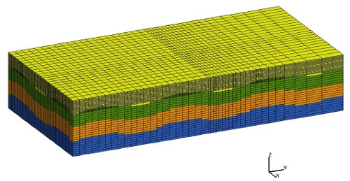
AVS data also contains material data. Each zone of different spacing is given a different material type in AVS. (The material numbers are chosen at random). A zone is an area with a certain type of spacing, created by the crossing of different regions in different axes. In the example figure, each zone is a different color.
Tracer3d formatted data gives only the location of the nodes, with no information about elements or connectivity.
Output Files
The output is written to a file called grid.inp. The file will be rewritten upon every run of the program. It might be useful to save the results of each trial.
The input parameters of the grid that were entered interactive or via the input file are saved to a file called input.tmp. To generate this same grid again without using the interactive mode, copy the file to another file name and type:
gridder <file_name
Non-Interactive Mode
Gridder can also be run with an input file that bypasses the questions of the interactive mode. The input file simply contains the answers to each of the questions that the interactive mode would have asked. For example see Input File that generated following picture
All input files require:
- number for dimensions/directions
- number of regions for x axis
Note
Next steps will be repeated byt he number of Dimenstions and by the order of Directions. For instance, if in previous step integer 6 was entered, then steps 3 to 7 will be repeated 2 times (for 2-D) starting for X direction and then continuing for Z direction.
- begin coordinate for the region
- end coordinate for the region. The coordinate to begin region must be < the coordinate to end the region
- number of divisions in the region. Here you can enter 0 for delta
- if you entered 0 in the previous step, enter the smallest delta. It must be > 0 and < region length. Otherwhise, enter number indicating type of spacing for first region
- (This step is optional.) If you entered geometric space (2) in previous step, then enter geometric factor, which should be > 0
- number indicating desired output format
Definitions and Examples of Some Terms
Regions
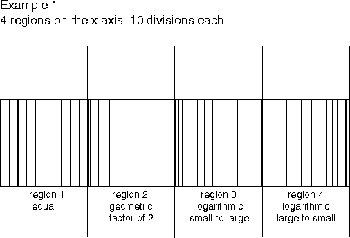
A region is a section of an axis with a beginning coordinate, an end coordinate, a number of divisions , and a number that indicates the type of spacing (equal geometric, logarithmic small to large, or logarithmic large to small). If any region in an axis has already been defined, the beginning border of the next region is automatically set equal to the end border of the previous region. Example 1 shows a set of coordinates on the x-axis with four different regions of the same size, each with ten divisions. The first consists of equall spaced nodes; the second of geometrically spaced nodes with a geometric factor of two; the third of logarithmically spaced nodes, small to large; and the fourth of logarithmically spaced nodes, large to small. This is actually a two-dimensional example, where the y-axis has only one region with one division in order to make the x divisions easier to visualize.
Zones
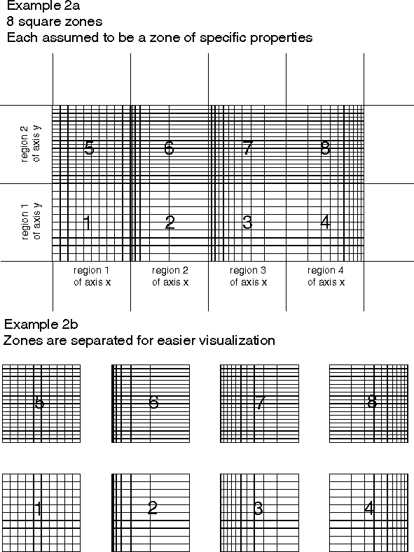
When there are multiple regions on two or more axes, the region boundaries cross, forming areas with a certain type of spacing in the x dimension, another type of spacing in the y dimension, and (if it is three-dimensional) another type of spacing in the z dimension. for example, in a two-dimensional grid, the region boundaries of the y-axis cross the region boundaries of the x-axis, dividing each region in the x-axis into areas with the same spacing in the x dimension, but each with a different type of spacing in the y dimension. These areas are referred to as zones. Example 2a has four regions on the x-axis, similar to example 1, but now there are two regions on the y-axis. The first has ten divisions, and the second has twenty divisions. Both have equally spaced nodes. The resulting cross of region borers creates eight zones. Example 2b is the same grid as example 2a, but it sohows the zones separated for easier visualization.
In AVS output, the zone number is used as the naterial number. If the user defines no properties for these material numbers, AVS will simply show each zone as a different color. Otherwise, the user can define these material properties to his or her preference, making each zone have different properties.
Equal Spacing
The user may pick one of four kinds of nodal spacing for each region. The simplest of these is referred to as equal spacing. Equal spacing of nodes simply means that the region is divided equally into the dgiven number of divisions. Each division is the same length. The formula for calculating the coordinates of equally spaced nodes can be found in Appendix 1.
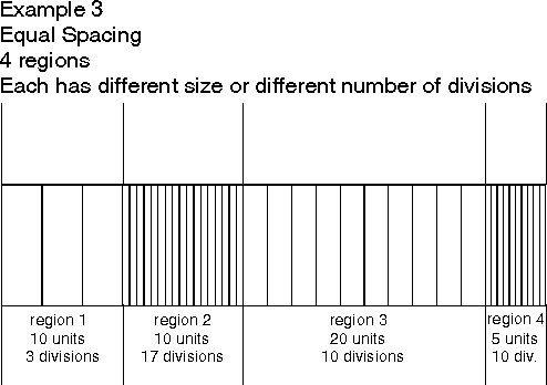
Example 3 shows a grid with four regions on the x-axis, each with equal spacing. The first two zones are both ten units long (last coordinate of zone munus first coordinate of zone=10) but the first has only three divisions while the second has seventeen. The third zone is only five units long but has ten divisions, and the fourth zone is twenty units long and also has ten divisions.
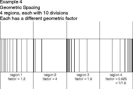
Geometric Spacing
In a geometrically spaced region, the distance between two consecutive nodes changes by a factor given by the user. TWhen geometric spacing is chosen, the user will be prompted for a “geometric factor” that determines this rate of change. For example, with a geometric factor of two, the largest division is twice the length of the previous division, which is twice the length of the division before that, etc. The coordinates become members of a geometric series. The actual formulas used to calculate the coordinates in a geometrically spaced series can be found in Appendix 1.
Example 4 shows some sample geometrically spaced regions. Each region is ten units long and has 10 divisions. The first has a geometric factor of 1.2, the second has a factor of 4, the third ahs a factor of 1.6, and the fourth has a factor of 0.625. If a user wants the distance between nodes to shrink by a given factor as opposed to growing by that factor, he or she can simply input the value of 1 divided by that factor (1/f) when prompted for a geometric factor. Zones 3 and 4 in Example 4 demonstrate this relationship. Zone 3 has a geometric factor of 1.6, and zone 4 has a geometric factor of 0.625 = 1/1.6. They have the same rate of change of distance between nodes, but in opposite directions (distances in zone 3 are growing from left to right while distances in zone 3 are shrinking from left to right.
A geometric factor of 1 would result in the equivalent of equal spacing.
Also notice that the smallest divisions becomes very small before the geometric factor gets very large at all. As this length decreses, accuracy decreases. I therefore recommend avoidance of large geometric factors as well as avoidance of very large numbers of divisions within a small region.
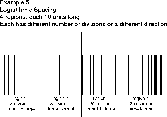
Logarithmic Spacing
In a region with logarithmic spacing, coordinates of nodes are determined as a function of a base 10 logarithm. Since by nature, logarithmic spacing results in smaller divisions growing to larger divisions as we move from left to right across the region, I have included a separate type of spacing that allws the user to assign “backwards” logarithmic spacing, where, from left to right, the divisions are larger and become smaller. Details of how logarithmic spacing is calculated can be found in Appendix 1.
Example 5 shows some sample regions with logarithmic spacing. There are 4 regions on the x-axis, each 10 units long. The first two have 5 divisions each, the first with spacing of small divisions to large and the second with large to small, and the last two have 30 divisions each, the third with small divisions to large and the fourth with large to small.
Limitations
Limited Number of Nodes and Regions
As the program stands now, there can be no more than 16385 nodes in any one axis, and no more than 500 regions. If desired, these limits can be easily changed in the source code. They are constants that are defined at the beginning of the code called MAXNODES and MAXZONES.
Accuracy
Coordinates are given with accuracy up to 6 significant digits. If the number of divisions becomes very large with respect to the size of the region, or if the geometric factor of a region with geometric spacing gets too large, the smallest divisions can become too small with respect to the other divisions in the grid, and accuracy decays. No more than 6 decimal digits difference in length of divisions can be calculated. I recommend avoidance of these practices that may result in verry small sized divisions.
Happy Gridding!
Appendix I
This appendix gives the formulas use to calculate the different kinds of spacing available from this grid generator, including equal spacing, geometric spacing, and logarithmic spacing. For all of the formulas given in this appendix, the following conventions will be used:
dx is the distance between first two consecutive nodes in region
n1 is the first coordinate in the region. This is entered by the user for the first region. For all subsequent regions, n1 is set equal to the last coordinate of the previous region.
n2 is the second coordinate in the region, etc..
nx is the last corrdinate in the region,
d is the number of divisions in the region
x is the total number of coordinates in region = d + 1.
f is the geometric factor.
L is the length of the region.
px is the percentage associated with node nx.
Equal Spacing
Equal spacing of nodes is calculated according to the following formula:
If the region being configured is the first region of the axis, n1 is entered as the “beginning coordinate of the region” by the user. Ptherwise, n1 is the same coordinate that ended the previous region. The program does not duplicate this coordinate as a separate node in the axis.
Geometric Spacing
Geometric spacing is calculated according to the following formula:
Logarithmic Spacing
To achieve logarithmic spacing, all cases are determined with respect to an analogous region starting at 1 and ending at 10. The code divides this temporary region equally into the given number of divisions, takes the logarighm of each of those numbers, and treats the resulting numbers as percentages of the size of the actual region. That is the reason for choosing the region from 1 to 10: log(1) = 0, and log(10) = 1. Therefore, the first coordinate of the region is placed at 0% of the way across the actual region (at the beginning), and the last node is placed at 100% of the way across the region (at the end). Let’s consider the simplest example:
Let’s say the user actually wants a region that starts at 1 and ends at 10, so we need no analogous region. Let’s also say the he or she wants 9 divisions. The code divides the region into 9 equally spaced divisions, giving us the coordinates 1, 2, 3, 4 .... 10. It then takes the log of each of these numbers, giving us the following percentages: (the code actually calculates the logarithms to 6 decimal points precision)
log(1) = 0% log(2) = 0.310 = 30.1% log(3) = 0.477 = 47.7% log(4) = 0.602 = 60.2% ... log(10) = 1 = 100% We now calculate the actual coordinates of the nodes by the following formula: nx = n1 + (px * L)
So for example,
The formula for logarithmic spacing, large to small, is similar: nx = n1 - (px*L), where n1 in this case is the last coordinate of the region, the end border.
Even if the example above had not begun at 1 and ended at 10, we would have followed the same procedure, dividing a region from 1 to 10 into the number of divisions given by the user, taking the logs of those numbers, and using them as percentage distances across the region.
Back to Gridder Home Page